CS 435: An Introduction to Deep Learning

Note: this summary serves as a quick refresh of information only, and not for in-depth study.

Introduction

• Deep learning is a sub-field of machine learning based on neural networks
• What makes Deep Learning so special now?
  • Data
    • Features Engineer VS Universal Learning Theory
  • Computation power
    • GPUs accelerates the training of the model, by having large number of simple cores which allow parallel computing through thousands of threads computing at a time.
  • Mathematics to choose the right model
    • Regularization

DFF (Deep Feed Forward networks)

• Deeper networks:
  • Use far fewer units per layer.
  • Far fewer parameters.
  • Often generalize to the test set.
  • Often harder to optimize.
• Activations functions
  • ReLU
    • Most common
    • Derivative is 1 or 0
  • Leaky ReLU
    • Slightly better than ReLU
      • No 0 slope
  • Sigmoid
    • No sensitivity for a large number of values
  • Tanh
    • Better than sigmoid because it has zero mean activations.
• Loss functions
  • Regression: Mean square error
  • Binary: Binary Cross entropy
  • Multi-class: Cross entropy
• Network optimization
  • Classical/Batch Gradient decent
    • In a highly multi-dimensional parameter space we should not worry about the local minima.
    • One step (update) after iterating all training examples (one epoch).
    • Issues:
      • Scalability
      • Step size (overshoot)
  • Mini-batch Gradient decent
    • Less oscilations than online GD
    • Faster than classical GD
  • Online/Streaming GD
    • Too many oscillations
    • One step for each training example
  • Gradient Decent with Momentum
    • Computes an exponentially weighted average of the gradients and uses that gradient to update the weights
    • More smooth
  • RMSProp
  • ADAM
    • Combines RMSProb and Momentum
    • Adds bias correction
• Learning rate decay is to slowly decrease the $\alpha$ as the number of epochs increases. (Avoid overshoot).

Regularization

• Parameter Norm Penalty
• Data augmentation
• Early Stopping
• Parameters tying and sharing
• Dropout
  
• What is the difference between bias and variance?
  • Bias is the expected error on training dataset.
  • Variance is the expected error on unseen dataset.
  • Model with high variance pays a lot of attention to training data and does not generalize on the data which it hasn’t seen before.

CNN

• Input: grid-like structure
• What’s new?
  • Make the forward function more efficient to implement
  • Vastly reduce the amount of parameters in the network
• Fully connected layers are wasteful and may lead to overfitting.

Architecture

• What does the Convolution try to do?
  • Calculate the correlation between the filter and the image.
• We learn filter weights
• Padding:
  • Same
  • Valid
• Non-Linearity: ReLU
  • To avoid saturation issues.
• Role of pooling:
  • Invariance to small transformations
  • Larger receptive fields (neurons see more of input)
• Stride > 1 is an aggressive compression
  • Instead, do the convolutions with stride of 1 and then combine using pooling
• Max pooling:
  • Often more accurate than average pooling (less information loss)
  • Hyperparameters: pool size, pool stride.
• CNNs properties:
  • Sparse Interactions
    • Input neuron affects only a few output neurons
    • Output neuron value depends on a few input neurons
  • Receptive Field: (Deeper units interact with larger portion of input)
  • Parameters Sharing (Parameter/weight is used in all input locations)
  • Equivariance: (equivariance to translation/offset, but not for scale or rotation)
  • Can work with inputs with variable sizes

Case Studies

• LeNet
• AlexNet
• VGG16
• ResNet
  • Uses skip connections to address very deep networks issues that lead to vanishing and exploding of gradients.
  • $ a^{[l + 1]} = g(z^{l+1} + a^{[l]})$
• Inception

Object detection

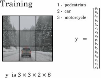
YOLO (State of the art)

• Solves object detection as regression problem.
• $y = [$Pc Xc Yc h w c1 c2 c3$]^T$
  • Pc: probability that there is object or not.
  • x, y, h, w: Bounding box boundries
  • c1, c2, c3: one hot encoding for classes.
• loss function: MSE
  • if Pc = 1: $ | \hat{y} - y |^2 $
  • else if Pc = 0: $ | \hat{y}_1 - y_1 |^2 $ (only first element as others are don’t cares)
• Problem: Most of the parameters in CNNs comes from the last FC layers.
  • Solution: Convert FC layer to convolution layer using 1x1 convolution operation.
• Problem: In Sliding window we need to apply the binary classifier to each window.
  • Solution: Use convolutions of the same size as the input. e.g need to take 4 windows output will be 2x2x4.

    

• Output will be conv of all sliding windows
  • Advantages:
    • Reduced computaion instead of classifying each window alone.
    • Shared Computation (Context)
• IoU (intersection over union) = $ \frac{area(intersection)}{area(union)} $, good if > 0.5
• Non-max suppression:
  1. Discard any BB (Boundry box) with $ P_c < 0.6 $
  2. Take BB with max $ P_c $ and add it to the output list
  3. Remove all BBs with $ IoU > 0.5 $
  4. Repeat until no BB left and return the output list.
• YOLO divides image into grid of cell (19 x 19)
• Problem: Detecting many objects at the same time in the same cell.
  • Solution: Anchor boxes.
• Anchor boxes
  • Each cell can detect up to number of anchor boxes.
  • Label vector is extended for each anchor box.

    

• One training sample will have vector for each cell, each vector has all anchor boxes values. i.e if we have 19x19 grid and 5 anchor boxes we will have $19 * 19 * 5 = 1805$ boxes for each training example.
• To know which object fits the best template (anchor box) we use IoU metric.
• We use the $P_c$ values to filter empty cells. (cells that has no objects).
• We do non-max supperesion on each class alone.

RNN

Architecture

• We apply the $ \tanh $ on hidden state and input.
  • Why tanh?
    • because it’s range is from [-1, 1] and hence we don’t lose the information of negative values.
  • Why not in CNNs?
    • In CNNs we are interested in maximum activations, thats why we do max pooling sometimes, and as we saw in some cases it’s better than average pooling.
• We apply (Sigmoid/Softmax/Linear) activations on output depending on the problem.
  • Named entity: Sigmoid
  • Language model (Probability distribution over words): softmax
  • regiression problem: Linear
• Why we need non-linearity in RNN (أصلا)?
  • To be able to do universal function approximation
  • Learn complex functions.
• Zero padding is a solution for varying network input length (time steps).
• One hot encoding is a solution for the different length in input of single RNN unit (e.g words).
• What makes RNN so special بقا?
  • Simply, The memory. When I feed the same input again we will have different output because hidden state (memory) will change.
• one-to-one RNNs: same as traditional networks.
• one-to-many RNNs: image captioning
• many-to-many RNNs: Sentiment analysis (Using word embeddings)
• many-to-many RNNs:
  • Same length: Named entity recognition
  • Different length: Machine translation
• What is the problem of Backprobagation through time in RNNs?
  • Exploding of gradients: solved using gradients clipping
  • Vanishing of gradients: solved using gates (GRU & LSTM)
• Why Exploding of gradients was not an issue in CNNs?
  • because there was no connections between neurons only between layers so the backprobagation was simpler than RNNs.
• What is language model?
  • Given words as input we output a probablity distribution over words that could come next.
• GRU unit (Simplifed) has 1 gate (Update gates) which controls the update of hidden state: \(C^{< t >} = \Gamma_u * \tilde{C}^{< t >} + (1-\Gamma_u) * C^{< t-1 >}\)
• GRU unit (Full) has two gates:
  • Update Gate: same as above $ (\Gamma_u) $
  • Reset Gate: whether to take previous state or not. (reset memory) $ (\Gamma_r) $
• LSTM unit has three gates:
  • Write Gate: Write/Use the input or not. $ c^{< t >} = \Gamma_u * \tilde{c}^{< t >} + \Gamma_f * c^{< t-1 >} $
  • Forget Gate: Forget previous input or not $ c^{< t >} = \Gamma_u * \tilde{c}^{< t >} + \Gamma_f * c^{< t-1 >} $
  • Read Gate: Read/Pass the output or not. $ a^{< t >} = \Gamma_o * c^{< t >} $
• All gates use sigmoid in their computaions
• Peehole variation of LSTM uses state $ C_t $ in their compuations instead of $ a_{t} $
• Coupled forget input gates variaiton uses one gate instead of write & forget gates: \(C_t = f_t * C_{t-1} + (1 - f_t) * \tilde{C}_t\)
• Bi-Directional RNNs is used to understand context from future and past, useful in named entity recognition probelms.
  • Issues?
    • Need full input before processing, hence can’t do real time processing.
• Deep RNNs … ¯\_(ツ)_/¯
• Regularization in RNNs:
  • L2
  • Dropout
    • Can only be done on input and output and not on recurrent connections. Why? Because we don’t want to remove memory!

NLP Apps

Word Emdedding

• We need word embedding to:
  • Avoid semantic ambiguity (Words that need context to understand them)
  • Avoid sparsity of input (one hot encoding) e.g 200 length instead of 10K!
  • Generalization + Share parameters
  • Understand relations between words. $ Women - Man + King = Queen $
• What was the problem in one-hot-encoding?
  • The distance between any two vectors is the same.
  • Cannot detect useful relations.
• How to train?
  • Unsepervised learning (Lots of data from web, wiki ..)
• How can we know the we got good embeddings?
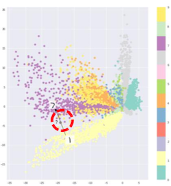
  • Visualization using t-SNE algorithm.
• NOTE: Word embedding is only useful for the tasks thet have small training sets e.g named entity recognition, hence not useful for Language Model and Machine Translation.
• Similarity functions in word embeddings:
  • Euclidean distance
  • Cosine Similarity (most used) ¯\_(ツ)_/¯ جربوها ونفعت
• $ W_{(300, 10K)} * o_{17 (10K, 1)} = e_{17 (300, 1)} $ Where $ W $ is the learned embedding matrix of size (embdedding length = 300 * vocabulary length = 10K)

Word Emdedding Algorithms

1. Language model
   • Remove one word (target) from sentence and predict it using the context (rest words in the sentence).
     • I want a glass of orange _____.
   • Can use target in the middle of sentece
     • I want a glass of orange _____ to go along with my cereal.
   • Can use one word as context (The previous word).
     • Oragnge _____.
   • Or Nearby word.
     • glass __.
     • This is the extension idea for word2vec. (skip gram model).
   • Loss function is the cross entropy between the netword output (softmax) and the target word one hot encoding vector.
   • What is the issue in this approach?
     • Complex FNN (too much parameters)
     • Computations of softmax is costly. (the summation term in denominator)
2. Skip grams (word2vec)
   • Computationally more efficient than language model.
   • What issues still exist here?
     • Computations of softmax, solved using:
   • hierarchical Softmax ( $ log_2 (| V |) $ instead of $ |V| = 10K $ )
   • Sample non-target words.
3. Negative sampling
   • Much more computationally efficient.
   • Differet approach than language model: binary classification.
     • Is target and context related or now.
   • (Orange, Juice) = 1
   • (Orange, King) = 0 * How do we generate labels in negative sampling? - For positive sample: Same as we did in lanugage model, we take one word as target and another word from context window as the context. - For K negative samples: We take any other words from vocabulary with the context word.
   • K is typically 5-20 for small dataset
   • 2-5 for large dataset * Problems in negative sampling: - Sample with word frequencies.
   • Stop words (a, the, and, ..) will occure the most. - Sample uniformally
   • No representative of the vocabulary. - Solution is to use the empirical formula. (In the lecture).
4. Glove algorithm
   • Glove combines the traditional NLP methods (Global matrix factorizaiton) and modern methods (Local context window).

Sentiment Analysis

• Problem: Lack of training data
• Solution: word embedding
• Idea: Average words embedding vectors and output softmax over the 5 review classes (1-5)
  • Problem?
    • Average causes loss of information (Negations words e.g not, never ..).
  • Solution?
    • many-to-one RNN. Save history and use gates to ignore any positive words if negation is encountered for example.

Debiasing

• Problem:
  • Man:Computer_Programmer & Woman:Homemaker
• Solution:
  • Move non-definitional words to be equi-distant from definitional words. (i.e project non-definitional words on the non-bias axis).
• Definitional words like Father, Mother ..
• Non-Definitional words like Doctor, Computer_Programmer ..

seq2seq

Encoder-Decoder models

• many-to-many RNNs
• Problem: find the most likely sequence \(argmax_{y< 1 > , ..., y< Ty >} P(y^{< 1 >}, .., y^{< Ty >} | x^{< 1 >}, .., x^{< Tx >})\)
• Solution:
  • Greedy Search
    • Select the most probable first word, then select the most probable second word given the first word and so on until < EOS >..
    • Not optimal, may be incorrect.
  • Exhaustive search
    • $ (|V|^n) $! where n is sentence length
  • Beam search
    • We take most probable B words first, then for each word we find the probabilities of ($ B * |V| $) posibilities and again select the most probable B words.
    • Always keep B choices in any step
    • Repeat until < EOS >
    • Issues?
      1. Multiplication of probabilities (numerical issues) $ argmax_y \prod_{t=1}^{T_y} P(y^{< t >} | x, y^{< 1 >}, .., y^{< t - 1 >}) $
      2. Favor shorter sentences
    • Solution?
      1. Take log $ argmax_y \sum_{t=1}^{T_y} log P(y^{< t >} | x, y^{< 1 >}, .., y^{< t - 1 >}) $
      2. divides by $ T_y^{\alpha} $: $ \frac{1}{T_y^{\alpha}} argmax_y \sum_{t=1}^{T_y} log P(y^{< t >} | x, y^{< 1 >}, .., y^{< t - 1 >}) $ $ 0 < \alpha < 1 $ typically 0.7
• Error analysis: checks if it is Beam Search that is causing error or the RNN. Should I increase the B or change the model.
  • If $ P(y^* | x) > \hat{P}(y^* | x) $
    • Beam search is at fault
  • If $ P(y^* | x) < \hat{P}(y^* | x) $
    • Model is at fault
• Performance Measure for Translation System
  • “Recall”: افتكرت قد ايه صح من الصح الكلي؟ = $ \frac{TP}{TP+FN} $
  • “Precession”: من اللي انا قلت عليه صح قد ايه فيه فعلا صح؟ = $ \frac{TP}{TP+FP} $
  • “Modified Precision”: $ \sum_{i=1}{\frac{clipped\_count_i}{count_i}} $
    • $ clipped\_count_i = max\_count(GT\_transalation1, GT\_transalation2) $
    • $ count_i = count(MT\_output)$
  • “Bleu Score”: $ BP * e^{\frac{1}{4} \sum_{n=1}^4 P_n} $
    • $ P_n $: Modified precesion over n-grams e.g. 1 word, 2 words …
    • $ BP $: Brevity penalty, to penalize short translation (as they usually will have high precision) A better Solution for this issue is attention models.

Attention models

• Attention models VS encoder-decoder models
  • Both allows any input length with any output length
  • Encoder-Decoder must process the entire sentence to get the output.
  • Attention models outptus on the go.

Attention model

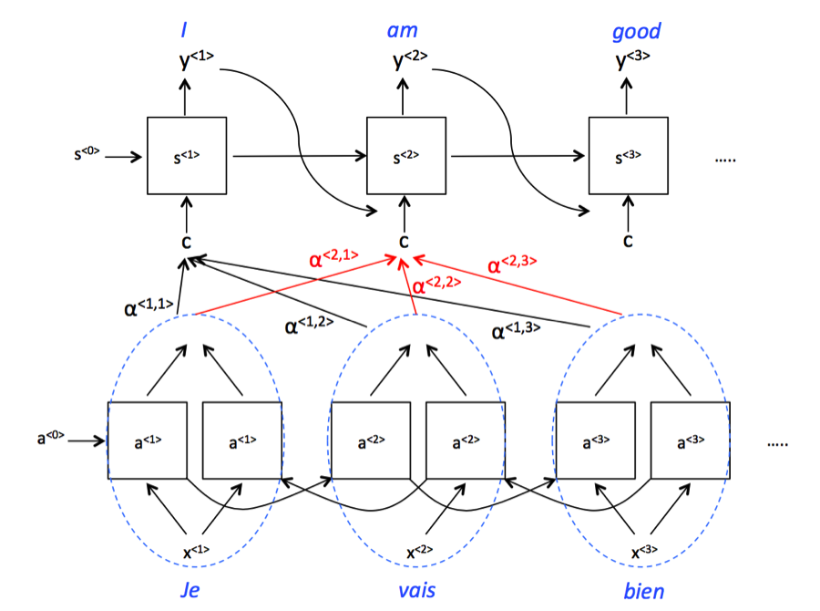
• Attention weights $ \alpha $ denote how much attention should be paid to each piece of the original sentence.

• The model is composed of two RNN networks. A bidirectional RNN to compute set of features for each of the input words and another RNN to generate the English translation. The input to the second RNN will be governed by the attention weights, which denote the context that is considered by every single word to compute the translation.

• Issues:
  • Computaions: If we have $T_x$ words as input and $T_y$ for the output, the total number of attention parameters is $ T_x * T_y $.
• Used in:
  • Normalize dates
  • Speech recognition (Input is an audio clip and the output is its transcript)

AE (Auto Encoder)

• Unsupervised approach
• Encoder-Decoder network
• Goal: learn subspase that represent the data (manifold learning) from a huge space. e.g $ 2^{1024*1024} $ for greyscale images of size 1024 * 1024.
• Usage:
  • Dimensionality reduction
  • Features extraction
• Is perfect reconstruction good?
  • No, it’s Same as overfitting. we don’t wan’t to overtrain the input.
  • So we avoid overtraining by enforcing the network to learn only important features.
• Two types of AE:
  • Over complete if $(h > input)$
    • May learn the trivial identity operation. Solution: regularization
  • Under complete $(h < input)$
    • Will enfore learning important features
• Parameters tying between encoder $(W)$ and decoder $(W^T)$
  • Why transpose?
    • One reason is that $W$ may not be a square matrix so we can’t take inverse. (هبد؟)
    • More here: https://datascience.stackexchange.com/questions/9769/why-is-reconstruction-in-autoencoders-using-the-same-activation-function-as-forw (عيش)
• Regularized AEs
  1. Sparse Autoencoders
     • loss fn = $ L(x, g(f(x))) + \Omega(h, x) $, where $ \Omega(h, x) = \lambda \sum_i | h_i | $
     • Helps avoid overtraining, so we can use over-complete AEs with regularization.
  2. Denoising Autoencoders
     • Add noise to input and try to undo this noise. (helps learn the manifold better)
     • noise can be:
       • Drop units randomly (every time)
       • Gaussian noise
  3. Penalizing Derivatives
     • For small change in input we don’t want a huge difference in output.
     • $ \Omega(h, x) = \lambda \sum_i |\nabla_x h_i |^2 $
     • AKA: Contractive autoencoder (CAE)
• Deep AE training strategy:
  1. Train shallow autoencoders (Stack of restricted Boltzmann machines (RBMs)).
  2. Unrolling: create deep AE.
  3. Fine-tune the whole network and remove parameters tying.
• Two way of visualizing what I learned:
  • Input all images and select the image that caused the maximum activation for each neuron.
    • Know what neuron learn.
  • Plot the weights of each neuron.
    • Intuition: if this image (Plot of weights) was an input (i.e $X = W$) it will cause the maximum activation for this neuron. since it will be $W^2+b$ which will have the max cos similarity.
• In localizaion AE is used to extract features for signals.

RL (Reinforcment Learning)

Classical RL

• RL is semi-supervised learning
• Exploration VS exploitation
  • exploration mean that we try different action which may lead to better reward
  • exploitaion goal is to maximize the reward using current info.
• RL approaches
  • policy based
  • values based
• The Q value for an action means the maximum reward we may get if we took this action.
• Q-learning is a value based approach
• Bellman equation: \(Q_{t+1}(s_t,a_t) = Q_{t}(s,a) + \alpha[\mathcal{R}_{t+1} + \gamma \max Q_t(s_{t+1}, a_{t+1}) - Q_{t}(s,a)]\)

• Can be written as exponential weighted average:

• $ \alpha $ detemins amount of exploration
  • $ \alpha = 1 $ is opimal for deterministic environment
• if $ \gamma = 1 $ we may not converge
• Main issue for classical RL is the huge space of the states.
  • Solution: DQN

DQN

• We have two options to represent our problem

  1. 

     Linear in number of actions

  2. 

     More effecient representation

• loss function: MSE (We have real values)
• DQN network: CNN
  • Same network for all games.
  • Different output depends on number of actions.
  • Reward clipping [1-, 1].
  • Input 4 frames at a time, Learn context (Is the ball in some frame moving up or down?).
  • Frames skipping. (Skip $k$ frames each 4 frames)
• Issues solved:
  1. Unknown target/Ground Truth (GT)
  2. $Q$ changes overtime, Chasing a moving target
  3. Input correlation, between frames. (Will cause a problem for SGD which work under the assumption that input is independent)
  4. Input/output correlation (The output determines the next input)
• How to get GT?
  • Step 1: propagate image to network, get the best action and execute it on emulator to get $S_{t+1}$ and $R$
  • Step 2: Calculate target: $ y = R + max_{a_{t+1}} Q(S_{t+1}, a_{t+1} | \Theta_i)$
• How to solve the moving target issue?
  • Have two networks $Q$ and $Q’$
    • Use $Q$ for training
    • Use $Q’$ for calculating the targets
    • $Q’ = Q$ for $C$ steps
• How to solve correlation issues?
  • Random shuffle from buffer (experience replay)

Generative Models

VAE (Variational Auto Encoder)

• We learn distribution explicitly (Vector of $\mu$’s and $ \sigma$’s)
• We use KL-Divergence as regularization term in our loss function to ensure the standard nomral distribution of our latent vairables. (hidden representaion)
• KL-Div: $ \sum p(x_i) = [ \log p(x_i) - \log q(x_i) ]$ is used to know the difference between two distributions (p, q) hence it limits the space between features encodings to minimize gaps in interpolation.

  

• KL-div: Expected difference info between two distributions.
• Loss function = reconstruction loss + regularization term
• The reconstruction loss helps learn semantics features.
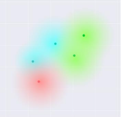
• If we use the regularization term alone, we may learn that all $\mu$’s and $ \sigma$’s are zeros. With the reconstruction loss term, it helps making latent variable far from each other, rather than all samples Centered around $\mu=0$.

  

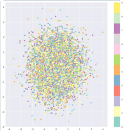
  Regularization alone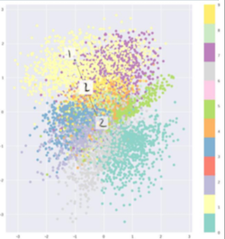

  

  Regularization + Reconstruction loss

• What is the difference between regularization term in standard AE and VAE?
  • In SAE:
    • Helps avoid overtraining.
  • In VAE:
    • Adds constraints on our distributions, and enforce that we have standard gaussian distribution.
• Why latent variables are independent?
  • Since the regulariztion term enforce that each one of them is standard normal, we get a vector of $\mu$’s and $\sigma$’s each is standard normal and independent, because by design and definition of our vector of $\mu$’s and $\sigma$’s we implicitly putting the non-diagonal values in the correlation matrix of latent variables to zero, so latent variables are uncorrelated.
• Problem of using SAE for generation?
  • Discontinuity
  • Less interpolation.

    

• What is the backprobagation issue in VAE and how it’s solved?
  • After we sample from the vector of $\mu$’s and $\sigma$’s we will get a scaler which cant take it’s derivative, hence we do the trick:
    • $x = \mu + \sigma sample(N(\mu, \sigma^2))$, (Equivalent and backpropagation-able)
    • The sampling layer is now linear function.

GANs (Generative Adversial Netowors)

• Implicitly learns the distribution
• Problem: Sample from complex distribution.
  • Solution: Use the inverse method.

    

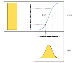
  • Instead of sampling from the distribution, we sample uniformally from the $CDF^{-1}$ of the distribution
  • Proof: Given: $ Y = CDF_x^{-1}(U)$ prove: $Y$~$X$
    • $CDF_Y(y) = P(Y \leq y)$ $ = P(CDF_X^{-1}(U) \leq y)$ , take $CDF_X$ for both sides $ = P(U \leq CDF_X(y))$, $($we know that $ = P(U \leq u) = u$ $)$ $ CDF_Y(y) = CDF_X(y) $ $Y$~$X$
• Lecture Note: we have 3 ways to proof that a random variable follows some distribution:
  • Moment generation function
  • CDF
  • PDF
• How can we get the $CDF^{-1}$?
  • We learn it using function approximation
  • So we can sample from easy distribution and the complex distribution is unknown.
• How to train?
  • Using two NN competing with each other (Generator VS discriminator).

    

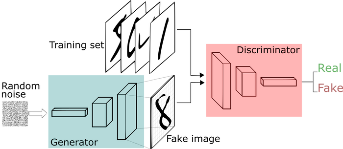
  • Discriminator: tries to identify real data from fakes created by the generator. (maximize real-fake diff)
  • Generator: Decode the random seed (noise) into an imitation of the data to try to trick the discriminator (minimize real-fake diff loss)
  • Update $\Theta_g$ to increase classification error
    • Gradient ascent over generator params
  • Update $\Theta_d$ to decrease classification error
    • Gradient descent over discriminator params
  • Train GAN via minmax game.
  • Algo:

    

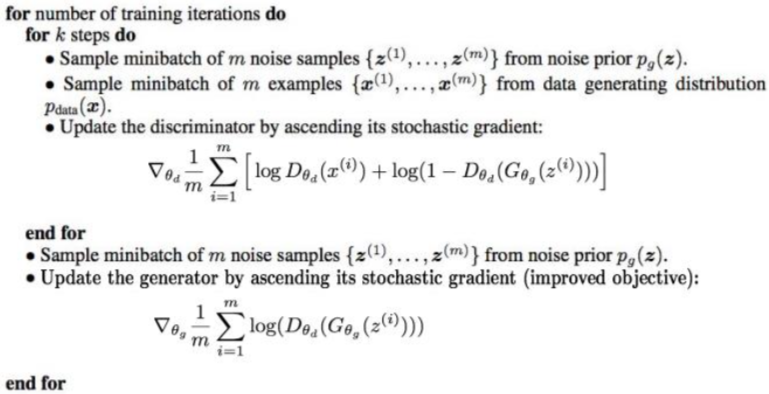
    • Note that the equations here are written so both discriminator and generator are maximizing cost function:
      • Discriminator wants to maximize objective s.t. $D(x)$ close to 1 (Real) and $D(G(z))$ close to 0 (Fake).
      • Generator wants to maximize objective s.t. $D(G(z))$ is close to 1 (Real)
      • Note: there is no -ve before the log

One Shot learning

• Goal: learn from few training examples.

Face recognition

• If we want to recognize from 4 faces, we will have CNN networds with 5 outpus (4 faces + 1 for otherwise)
• Two issues:
  • Few samples: poor performance (CNNs need a lot of data)
  • Change the output length everytime a new face is added in DB. (Retrain network)
• Solution:
  • Convert to matching problem
  • learn distance function $ d(img1, img2) > threshold $
• Face Verification
  • Whether the image of the claimed person or not (True/False)
• Face Recognition
  • Which face/ID does an input image belongs to.
  • Can be performed using Face Verification

• Binary classifier approach

  • 

    Binary classifier

  • We can precompute images features to enhance the model.
  • We have parameter tying.
  • We generate the training examples by sampling from matched images for postive examples and non-matched images for negative examples, problem?
  • Unblalanced data. solution?
  • Sample from non-matched image, only take the most critical/important images.
• Siamese networks
  • Problem in Triplet loss:
    • $ |f(A) - f(P)|^2 - |f(A) - f(N)|^2 <= 0 $
    • Can learn trivial solution. $ f(img) = 0 $
    • Solution: add margin $ \alpha $
      • $ |f(A) - f(P)|^2 - |f(A) - f(N)|^2 + \alpha <= 0 $
  • $ L(A, P, N) = max(triplet\_loss, 0) $
  • $ J = \sum_{i=1}^m L(A^i, P^i, N^i) $
  • Given K persons with two images each, we will have:
    • $K$ positive examples (matched images)
    • $ K^2 $ negative examples (non-matched images)
  • NOTE: Always choose triplets that hard to train on (عشان الصينيين مثلا)
    • $ d(A, P) \approx d(A, N) $

Neural Style Transfer

• Input: Content, style images
• Output: Generated image
• Goal: Modify the content to have the same style as the Style image
• How to capture style, and content in CNNs?
  • Content: using activations of layer $L$
    • if $L = 1$ match exactly the content (Layer captures the details)
    • More deeper, more complex/high features.
  • Style: (Correlations) between filters in style and generated filters (in same layer)
    • intuition: To make some filter in style image is correlated with filters in generated image, hence follow it’s style.
• Training:
  • Initialize G randomly
  • $ J(G) = \alpha J_{content}(C, G) + \beta J_{style}(S, G) $
  • Gradient Decent: $ G = G - \frac{\delta J(G)}{\delta G}$