Train/Dev/Test Sets
Sometimes you need to test different algorithms (models) on your data, doing so on such big data can be time consuming, so the best way to do this is divide your data into train, dev and test set.
- train set used for training and learning the parameters.
- dev set for model selection.
-
test set for testing the final model (the selected model) that is already trained.
- other names for dev set:
- development set
- hold-out set
- cross-validation set
- for big data it’s ok to divide your data like this -> 98% (train), 1% (dev), 1% (test).
- make sure your dev and test set comes from the same distribution
- not having test set might be ok only train/dev sets.
Yes, the separation of test and dev set was meant to only get an unbiased error estimate of the final model.
Bias and Variance
Recall that
- high bias means under-fitting
- high variance means overfitting
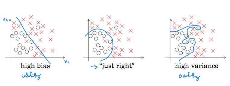
If we had two features \(x1, x2\) we can easily plot the decision boundary and know if we have high bias or high variance, but for larger features we will use the the train and dev set errors
| Train set error | dev set error | |
|---|---|---|
| 1% | 11% | this indicates that we have overfitting on the train set (high variance) |
| 15% | 16% | this indicates underfitting (high bias) |
| 15% | 30% | high bias and high variance |
| 0.5% | 1% | low bias and low variance |
NOTE: we alway assume that the human error is 0% which is also called base error, if the base error is something like 15% then for the second example it wouldn’t be underfitting.
TROUBLESHOOTING
-Train for longer time, use another algorithms.
- Search about other architectures online."]; B--> |No| D{High variance}; D--> |Yes| E["-Get more data (may be expensive)
- Use regularization.
-Search about other architecture."]; D--> |No| F[COOL!];
** bias and variance tradeoff
Regularization
Sometimes it’s expensive to get more data to solve high variance problem, regularization would be your best option.
L2 Regularization:
Recall: in logistic regression
\[J(W, b) = 1/m \sum_{i=1}^m \mathcal{L}(\widehat{y}, y^{i}) + \dfrac{\lambda}{2m} \Vert w \Vert^2_2 + \underline{\dfrac{\lambda}{2m}b^2}\]- This is called L2 regularization.
- note that the last term can be ignored
in Neural Networks: \(J(W_{[1]}, b_{[1]}, ..., W_{[L]},b_{[L]}) = 1/m \sum_{i=1}^m \mathcal{L}(\widehat{y}, y^{(i)}) + \dfrac{\lambda}{2m} \sum_{l} \sum_{k} \sum_{j} \Vert w_{kj}^{[l]} \Vert^2_F\)
- \(F\) stands for Forbenius.
- regularization makes weights smaller (weight decay).
Adding the penality to weights will shrink or OFF some nerouns which will make the architecture more simpler. Also, since
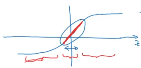
\[z^{[l]} = w^{[l]}*a^{[l-1]} + b^{l}\]shrinking weights will results in small \(z\) so the activation function say it’s \(tanh(z)\) will be linear at small values of \(z\) which is simpler and will not cause overfitting.
Important Note: Don’t forget to update the \(J\) forumula when plotting the \(J\) against the # of iterations
(\(J_{regularized} = J_{old} + regularization\))
Dropout regularization:
Randomly shutodown neurons in each layer.
Steps:
D_l = np.random.rand(A_l.shape[0], A_l.shape[1])
D_l = D_l < keep_prob
A_l = np.multiply(a3, d3)
A_l /= keep_prob
- in line 1
D_lis the dropout vector of layerl - in line 2
keep_probis the probability that some hidden unit will be kept, so ifkeep_prob = 0.8there is 0.2 chance of eliminating hidden units. - in line 3 we used element wise multiplication to shutdown some neurons.
- Finally in line 4 we scale the value of neurons that are kept by keep_prob since not all neurons of this layer will contribute to the output of this layer now.
We don’t apply dropout at test time because this adds noise to predictions, only apply it during training.
Other regularizatin methods
- Data augmentation (like flipping or rotating the images to make more data)
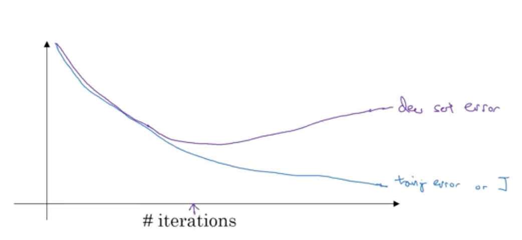
- Early stopping (Plot training set error with dev set error. when dev set error start rising, stop.)
Vanishing/Exploding gradients
When calculating the derivatives it can very small or very large, and this makes training difficult. a partial solutio of this problem is random initialization for the weights:
-
Well choosen initialization can speed up the convergance of gradient descent, and prouces good acuracy results.
-
There are different types of initialization:
-
Zeros initializatin: Network fails to break symetry, that means that every neuron in each layer will learn the same thing, the network is no powerful than a linear classifier such as logistic regression, it’s just like training a neurol network with only 1 neuron for every layer.
- Random initializatin: Breaks symetry, but don’t use large values, because this slows down the obtimization.
-
He initiliazation: Good for Relu activation functions.
\[\sqrt{\dfrac{2}{n^{[l-1]}}}\] -
Xavier initializatin: Good for tanh activation functions.
\[\sqrt{\dfrac{1}{n^{[l-1]}}}\]and sometimes this is used:
\[\sqrt{\dfrac{1}{n^{[l-1]} * n^{l}}}\]
-
Gradient Checking
Very usefull to find bugs in your gradient implemenetation.
- Gradient checking is slow so we don’t run it at every iterations in training. only few times to make sure the gradients is correct.
- Gradient checking doesn’t work with dropout, so don’t apply dropout which running it.
Resources: Deep Learning Specialization on Coursera, by Andrew Ng

Leave a Comment