In this week you will:
- learn different optimization methods such as (Stochastic) Gradient Descent, Momentum, RMSProp and Adam.
- Use random minibatches to accelerate the convergence and improve the optimization.
- Know the benefits of learning rate decay and apply it to your optimization.
Gradient Descent
Recall the update rule for gradient descent:
for \(l\) in \(L\):
\[W^{[l]} = W^{[l]} - \alpha \text{ } dW^{[l]} \tag{1}\] \[b^{[l]} = b^{[l]} - \alpha \text{ } db^{[l]} \tag{2}\]Where:
\(W: \text{ Weights} \)
\( b: \text{ biases} \)
\( \alpha: \text{ learning rate} \)
\( l: \text{ layer number} \)
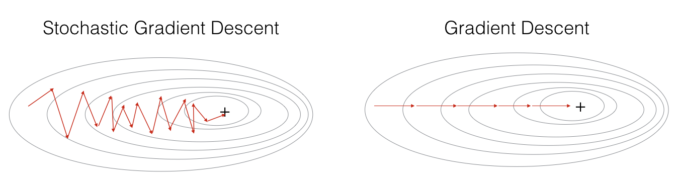
Batch Gradient Descent
- We update parameter every m example.
- We take gradient steps with respect to all \(m\) examples on each step.
- Equivalent to mini-batch gradient descent but with mini-batch size of \(m\).
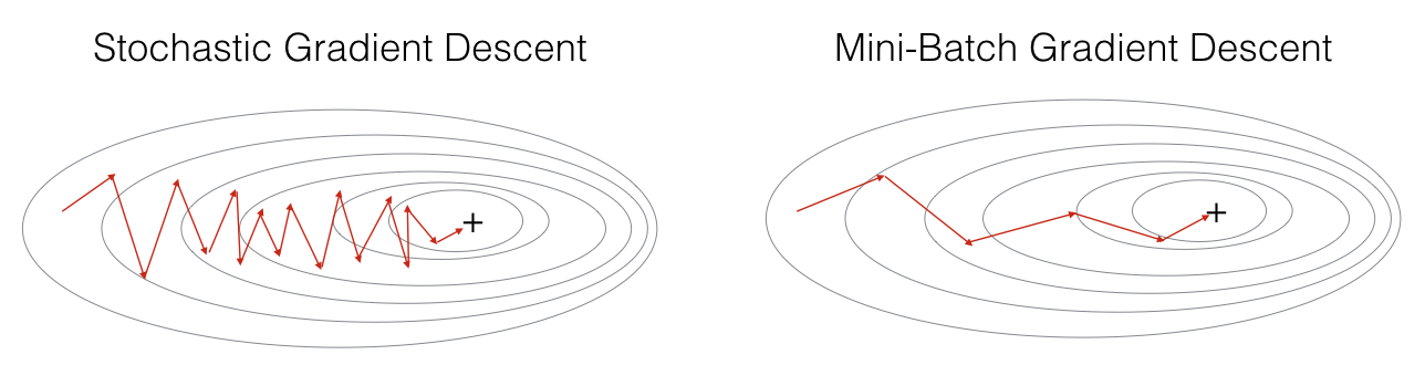
Stochastic Gradient Descent
- We compute gradients on one training example.
- We update parameter every 1 example.
- Equivalent to mini-batch gradient descent but with mini-batch size of \(1\).
Mini-batch Gradient Descent
- we update parameter every subset of examples.
- mini-batch size is between \(1\) and \(m\).
- It’s better to choose the mini-batch size to be powers of 2.
- it’s build in two steps:
- Shuffling (To ensures that examples will be split randomly into different mini-batches).
- Partition
- Note that the number of training examples is not always divisible by mini_batch_size.
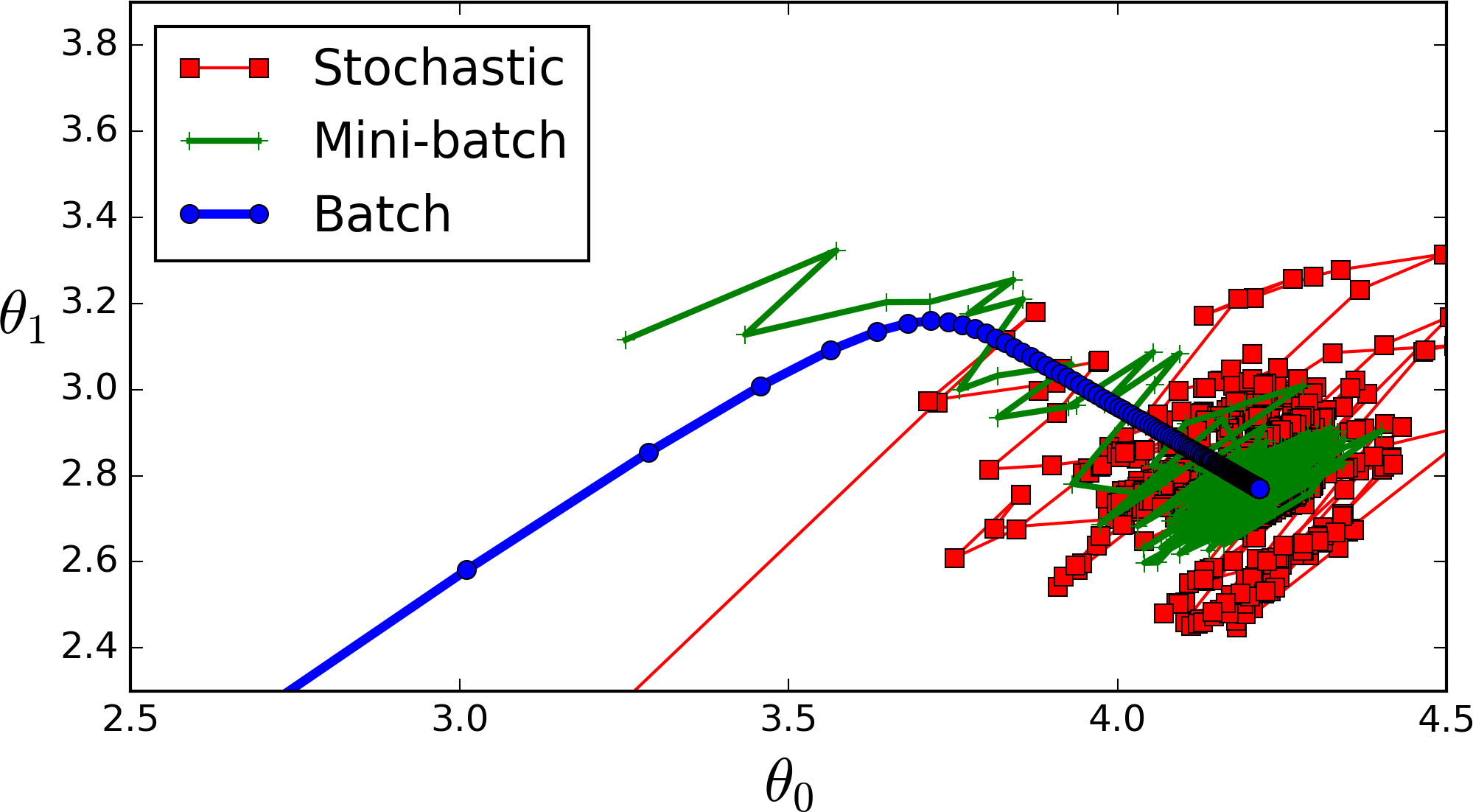
Extra: Here is a comparison that combines the three algorithms.
Gradient descent with momentum
- Using momentum can reduce the oscilation of mini-batch path toward convergence.
- Based on exponentially weigted averages.
- Takes into account past gradients to smooth out the update path.
- Direction of previous gradients is stored in \(v\) which can be seen as the velocity of a ball rolling down the pow.
- Velocities are initialized with zeros, that’s why the algorithms takes some time (few iterations) to warm up.
- If \(\beta = 0 \) this will be the standard gradient descent.
- beta is another hyperparamter that could be tuned, to reduce the value of cost funcion \(J\).
- The larger beta is the smother the path toward converence get, because more past gradient is taken into account.
- Common values for \(\beta\) is between 0.8 and 0.999.
- 0.9 is often resonable choice if you don’t want to tune it.
- Momentum can be applied with batch gradient descent, mini-batch gradient descent or stochastic gradient descent.

Momentum update rule:
for \(l\) in \(L\):
\[\begin{cases} v_{dW^{[l]}} = \beta v_{dW^{[l]}} + (1 - \beta) dW^{[l]} \\ W^{[l]} = W^{[l]} - \alpha v_{dW^{[l]}} \end{cases}\tag{3}\] \[\begin{cases} v_{db^{[l]}} = \beta v_{db^{[l]}} + (1 - \beta) db^{[l]} \\ b^{[l]} = b^{[l]} - \alpha v_{db^{[l]}} \end{cases}\tag{4}\]Where:
\(\beta: \text{ momentum} \)
\(v: \text{ velocity} \)
RMSProp
Surprisingly RMSProp was not introduced in some reasearch paper but a course in Coursera by Geoff Hinton!
\[s_{dW^{[l]}} = \beta_2 s_{dW^{[l]}} + (1 - \beta_2)(dW^{[l]})^2\] \[W^{[l]} = W^{[l]} - \alpha \frac{dW^{[l]}}{\sqrt{s_{dW^{[l]}} + \varepsilon}}\]- \(\varepsilon\) is to avoid the division by zero.
- RMSProp stands for root mean squared prop.
Adam optimization algorithm
- Combines the advantages of RMSProb and Momentum
- We have two variables \(v,s\) that keeps track of the past information.
How does it work?
Simply it:
- Calculates an exponentially weighted average of past gradients, and stores it in variables v (before bias correction) and vcorrected (with bias correction).
- Calculates an exponentially weighted average of the squares of the past gradients, and stores it in variables s (before bias correction) and scorrected (with bias correction).
- Updates parameters in a direction based on combining information from “1” and “2”.
The update rule is:
\(\text{for } l = 1, …, L:\)
\[\begin{cases} v_{dW^{[l]}} = \beta_1 v_{dW^{[l]}} + (1 - \beta_1) \frac{\partial \mathcal{J} }{ \partial W^{[l]} } \\ v^{corrected}_{dW^{[l]}} = \frac{v_{dW^{[l]}}}{1 - (\beta_1)^t} \\ s_{dW^{[l]}} = \beta_2 s_{dW^{[l]}} + (1 - \beta_2) (\frac{\partial \mathcal{J} }{\partial W^{[l]} })^2 \\ s^{corrected}_{dW^{[l]}} = \frac{s_{dW^{[l]}}}{1 - (\beta_1)^t} \\ W^{[l]} = W^{[l]} - \alpha \frac{v^{corrected}_{dW^{[l]}}}{\sqrt{s^{corrected}_{dW^{[l]}}} + \varepsilon} \end{cases}\]Where:
- \(t\) counts the number of steps taken of Adam
- L is the number of layers
- \(\beta_1\) and \(\beta_2\) are hyperparameters that control the two exponentially weighted averages.
- \(\varepsilon\) is a very small number to avoid dividing by zero often \(10^{-8}\)
Learning rate decay
Sometimes you need decrease the learning rate especially when you are about to reach convergence.
one way is:
\[\alpha = \frac{1}{1+decay-rate * epoch-num} \alpha_0\]Where
- \(\alpha_0 \): The initial learning rate.
- decay-rate is another hyperparamter you need to tune.
Other learning rate decay methods:
- \( \alpha = 0.95^{epoch-num} \alpha_0 \) (exponintially decay)
- \( \alpha = \frac{k}{\sqrt{epoch-num}} \alpha_0 \)
- And others ..
Notes:
- In linear algebra terms, m[:,n] is taking the nth column vector of the matrix m so taking the first 3 examples in input data X, X[:, 0 : 3]. (slicing). (important for programming assignment)
- Different optimization algorithms can leads to different accuracy so it’s important to always choose a good one.
- One epoch passes through all the \(m\) training examples whether you use batch, stochastic or mini-batch.
- Inside an epoch (iteration) you loop m times, 1 times or t times for stochastic, batch or mini-batches respectivaly.
- Very useful article: http://ruder.io/optimizing-gradient-descent/index.html
Resources: Deep Learning Specialization on Coursera, by Andrew Ng

Leave a Comment