Coursera deep learning specialization by Andrew Ng [Course 1 - Week 4]

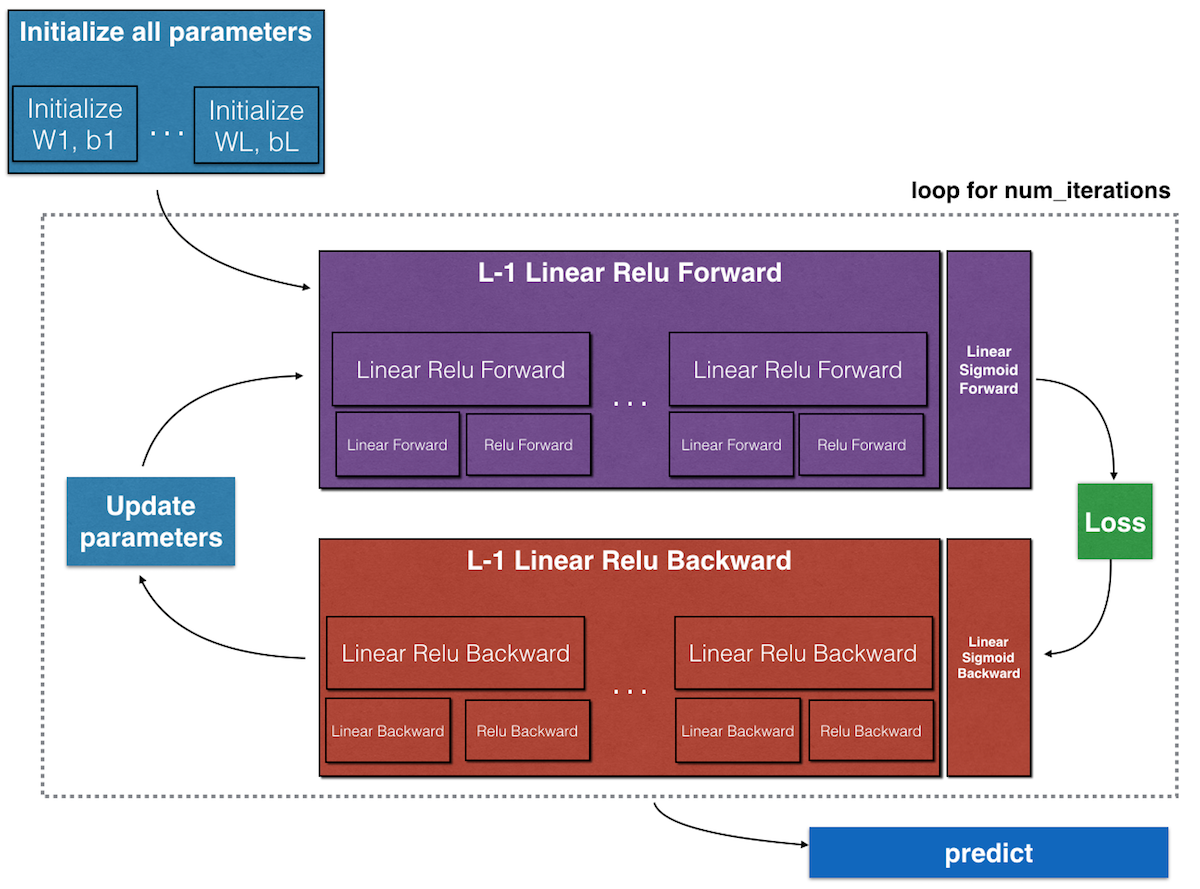
Step 1: Initialize parameters

• The bias vectors are initialized with zeros.
• The weights matrices are initialized with small random variables

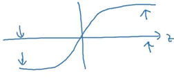
    np.random.randn(d1, d2) * 0.01
  

  0.01 can also be a variable that is chosen later but it’s not widely common. Choosing a big constant will affect the speed of gradient descent algorithm in some activation function like tanh(z) so the values will be either very small or very big and hence the gradients will be close to zero and will slow the algorithm.

tanh(z)

Step 2: Implement forward propagation

• compute \(Z^{[l]}\) and \(A^{[l]}\) for all layers
• linear forward (compute \(Z\))
• activation forward (compute \(A\))

Step 3: Compute cost function (\(J\))

• this is not included in the computations but it’s very useful for debugging and visualization.

Step 4: Implement backward propagation

• Use cached values from forward propagation to compute the gradients
• Linear backward (compute dW, db, dA_prev)
• Activation backward (com)

Step 5: Update parameters

• Update the parameters using the gradients computer in step 4.

    theta = theta - alpha * dtheta
  

  Where alpha is the learning_rate and dtheta is the derivative of cost function J with respect to theta.

Step 6: put step 2-5 into for loop num_iterations (gradient descent)

Step 7: Predict

(The model's structure is [LINEAR -> RELU] × (L-1) -> LINEAR -> SIGMOID. I.e., it has L−1 layers using a ReLU activation function followed by an output layer with a sigmoid activation function.)

---

Notes:

• we don’t calculate the input layer in the total number of NN layers
• The input layer is layer zero (\(l\) = 0)
• \(A_{0} = X\)
• \(n_{0} = n_x\)
• \(A_L = \widehat{Y}\)
• 1 layer NN is actually logistic regression (shallow NN)
• More than 2 layer NN is called (Deep NN)
• In deep learning, the “[LINEAR->ACTIVATION]” (compute the forward linear step followed by forward activation step) computation is counted as a single layer in the neural network, not two layers.

Resources: Deep Learning Specialization on Coursera, by Andrew Ng